Chapter7 Vectors

Vectors are the simplest data structure in R. A vector is simply a collection of elements arranged in a specific order, and we can imagine it similarly to the representation shown in Figure 7.1.

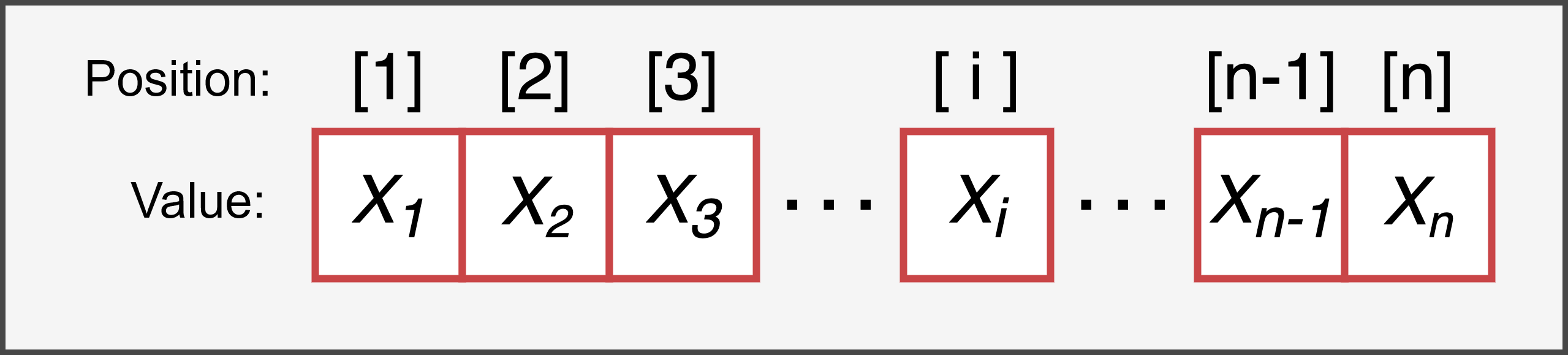
Figure 7.1: Representation of the structure of a vector of length n

Two important characteristics of a vector are:

• la Length - the number of elements that make up the vector.
• la Type - the type of data that makes up the vector. A vector must be composed of elements all of the same type; therefore, there are different types of vectors depending on the data type (numeric, integer, logical, or character values).

It’s also important to emphasize that each element of a vector is characterized by:

• un a value - the value of the element, which can be anything, such as a number or a string of characters.
• un a position index - a positive integer that identifies its position within the vector.

Thus, vectors \(x\) and \(y\) defined as: \[ x = [1, 3, 5];\ \ \ y = [3, 1, 5], \] though containing the same elements, are not identical because they differ in their order. This illustrates how the order of elements is crucial in evaluating a vector.

Now, let’s see how to create vectors in R and perform common operations such as selection and manipulation. We will then explore vector characteristics by examining their different types.

7.1 Creation

We’ve already encountered vectors in previous chapters, as even variables with a single value are simply vectors of length 1. However, to create vectors with multiple elements, we use the c() command, meaning “combine”, specifying the elements in the desired order and separating them with commas. The syntax is as follows:

vector_name = c(x_1, x_2, x_3, ..., x_n)

Note that the elements of a vector must all be of the same type, for example, numeric or character values.

Alternatively, any function that returns a sequence of values as a vector can be used. Some of the most commonly used functions for creating sequences are:

• <from>:<to> - Generates a sequence of increasing (or decreasing) numeric values from (<from>) to (<to>) in steps of 1 (o -1 ).

# increasing sequence
1:5
## [1] 1 2 3 4 5

# decreasing sequence
2:-2
## [1]  2  1  0 -1 -2

# sequence with decimal values
5.3:10
## [1] 5.3 6.3 7.3 8.3 9.3

• seq(from = , to = , by = , length.out = ) - Generates a regular sequence of numeric values between from and to with increments specified by by, or with a total length specified by length.out (see ?seq() for more details).

# sequence with increments of 2
seq(from = 0, to = 10, by = 2)
## [1]  0  2  4  6  8 10

# sequence with 5 elements
seq(from = 0, to = 1, length.out = 5)
## [1] 0.00 0.25 0.50 0.75 1.00

• rep(x, times = , each = ) - Generates a sequence by repeating the values in x. The values in x can be repeated multiple times in order using times or each value can be repeated multiple times using each (see ?rep() for more details).

# repeated sequence
rep(c("foo", "bar"), times = 3)
## [1] "foo" "bar" "foo" "bar" "foo" "bar"

# sequence with repeated elements
rep(1:3, each = 2)
## [1] 1 1 2 2 3 3

Exercises

Familiarize yourself with vector creation (solutions):

1. Create the vector x containing the numbers 4, 6, 12, 34, 8.
2. Create the vector y containing all the even numbers between 1 and 25 (?seq()).
3. Create the vector z containing the first 10 multiples of 7 starting from 13 (?seq()).
4. Create the vector s where the letters "A", "B", and "C" are repeated in the same order 4 times (?rep()).
5. Create the vector t where the letters "A", "B", and "C" are each repeated 4 times (?rep()).
6. Generate the following output with minimal code.

## [1] "foo" "foo" "bar" "bar" "foo" "foo" "bar" "bar"

7.2 Selecting Elements

Once a vector is created, you may need to select one or more of its elements. In R, to select elements from a vector, square brackets [] are used after the vector name, with the position index of the desired elements inside the brackets:

vector_name[<position-index>]

Be careful not to specify the value of the desired element, but its position index. For example:

# given the vector
my_numbers = c(2,4,6,8)

# to select the value 4, use its position index, which is 2
my_numbers[2]
## [1] 4

# If you use its value (4), 
# you'll get the element in the 4th position
my_numbers[4]
## [1] 8

To select multiple elements, list all the desired position indices within the square brackets. Note that you can’t simply provide individual numbers; they must be enclosed in a vector, for example, using the c() function. Essentially, you use a vector of indices to select the elements from the original vector.

# INCORRECT selection of multiple values
my_numbers[1,2,3]
## Error in my_numbers[1, 2, 3]: incorrect number of dimensions

# CORRECT selection of multiple values
my_numbers[c(1,2,3)]
## [1] 2 4 6
my_numbers[1:3]
## [1] 2 4 6

Note that selecting elements does not modify the original vector. If you want to keep the changes, you need to save the result of the selection.

my_words = c("foo", "bar", "baz", "qux")

# Selecting the first two elements
my_words[1:2]
## [1] "foo" "bar"

# The original vector still has all the elements
my_words
## [1] "foo" "bar" "baz" "qux"

# Save the result
my_words = my_words[1:2]
my_words
## [1] "foo" "bar"

What happens if you use a position index greater than the number of elements in your vector?

# My vector
my_numbers = c(2,4,6,8)

my_numbers[10]
## [1] NA

R doesn’t return an error but gives the value NA (Not Available) to indicate that no value is available.

Let’s also explore other special behaviors or possible errors in element selection:

• The position index must be a numeric value, not a character.

# INCORRECT selection of multiple values
my_numbers["3"]
## [1] NA

# CORRECT selection of multiple values
my_numbers[3]
## [1] 6

• Decimal numbers are ignored, not rounded.

my_numbers[2.2]
## [1] 4
my_numbers[2.8]
## [1] 4

• Using the value 0 returns an empty vector.

my_numbers[0]
## numeric(0)

7.2.1 Advanced Uses of Selection

Let’s now look at some advanced uses of vector element selection. Specifically, we will learn how to:

• use relational and logical operators to select elements from a vector
• change the order of elements
• create new combinations
• replace elements
• remove elements

Relational and Logical Operators

A useful function is selecting elements from a vector that meet a certain condition. To do this, you specify the condition inside square brackets using relational and logical operators (see Chapter 3.2).

For example, we can select all elements greater than a certain value from a numeric vector, or select all elements equal to a specific string from a character vector.

# Numeric vector - select elements greater than 0
my_numbers = -5:5
my_numbers[my_numbers >= 0]
## [1] 0 1 2 3 4 5

# Character vector - select elements equal to "bar"
my_words = rep(c("foo", "bar"), times = 4)
my_words[my_words == "bar"]
## [1] "bar" "bar" "bar" "bar"

To better understand this process, it’s important to note that there are two distinct steps in the same command:

• Logical vector (see Chapter 7.4.4) - When a vector is evaluated in a condition, R returns a new vector containing the answer (TRUE or FALSE) for each element of the original vector.
• Selection - We use the resulting logical vector to select elements from the original vector. Elements associated with TRUE are selected, while those associated with FALSE are discarded.

We can make these two steps explicit in the following code:

# Logical vector
condition = my_words=="bar"
condition
## [1] FALSE  TRUE FALSE  TRUE FALSE  TRUE FALSE  TRUE

# Selection
my_words[condition]
## [1] "bar" "bar" "bar" "bar"

Sorting Elements

Position indices can be used to sort the elements of a vector according to your needs.

messy_vector = c(5,1,7,3)

# Reorder the elements
messy_vector[c(4,2,3,1)]
## [1] 3 1 7 5

# Sort elements in ascending order
messy_vector[c(2,4,1,3)]
## [1] 1 3 5 7

To sort elements in ascending or descending order (either alphabetically or numerically), you can use the sort() function, specifying the decreasing argument. See the help page of the function for more information (?sort()).

# Alphabetical order
my_letters = c("cb", "bc", "ab", "ba", "cb", "ab")
sort(my_letters)
## [1] "ab" "ab" "ba" "bc" "cb" "cb"

# Descending order
sort(messy_vector, decreasing = TRUE)
## [1] 7 5 3 1

Note that there is also the order() function, but it is a false-friend because it does not directly provide a vector with sorted elements but instead returns the position indices for reordering the elements (?order()). See how to use this function in the following example:

# Position indices for reordering elements
order(messy_vector)
## [1] 2 4 1 3
# Reorder the vector using the position indices
messy_vector[order(messy_vector)]
## [1] 1 3 5 7

Combinations of Elements

The same position indices can be used multiple times to repeat elements in the desired combinations, forming a new vector.

my_numbers = c(5,6,7,8)
# Obtain a new vector with the desired combination
my_numbers[c(1,2,2,3,3,3,4)]
## [1] 5 6 6 7 7 7 8

Replacing Elements

An important use of indices is modifying an element in a vector. To replace an old value with a new one, you can use the assign function (<- or =), as in the following example:

my_names = c("Andrea", "Bianca", "Carlo")

# Replace the name "Bianca" with "Beatrice"
my_names[2] = "Beatrice"
my_names
## [1] "Andrea"   "Beatrice" "Carlo"

To replace a value, you specify the value to modify on the left of the assignment operator, and the new value on the right. Note that this operation can also be used to add new elements to the vector.

my_names[4]
## [1] NA

# Add the name "Daniela"
my_names[4] = "Daniela"
my_names
## [1] "Andrea"   "Beatrice" "Carlo"    "Daniela"

Removing Elements

To remove elements from a vector, specify the position indices of the elements to remove inside square brackets, preceded by the - (minus) operator. If removing multiple elements, you can use the minus operator only before the c() function, for example, x[c(-2,-4)] becomes x[-c(2,4)].

my_words = c("foo", "bar", "baz", "qux")

# Remove "bar"
my_words[-2]
## [1] "foo" "baz" "qux"

# Remove "foo" and "baz"
my_words[-c(1,3)]   # alternatively, my_words[c(-1, -3)]
## [1] "bar" "qux"

Note that removing elements is still a selection operation. Therefore, you need to save the result if you want to keep the changes.

# Remove  "foo" and "baz"
my_words[-c(1,3)]
## [1] "bar" "qux"

# The original vector still has all elements
my_words
## [1] "foo" "bar" "baz" "qux"

# Save the results
my_words = my_words[-c(1,3)]
my_words
## [1] "bar" "qux"

7.2.1.1 which()

The which() function is very useful for obtaining the position within a vector that meets a certain logical condition. For instance, if we want to know the positions of values greater than 5 in a numeric vector, we can use the function which(x > 5), where x is our numeric vector.

##  [1] FALSE FALSE  TRUE  TRUE FALSE FALSE  TRUE FALSE FALSE FALSE
## [1] 3 4 7

As you can see, the which() function essentially returns the position (not the value) where the tested condition is TRUE. It’s important to note that these two pieces of code are equivalent:

## [1] 10.760911  7.608606  5.829283
## [1] 10.760911  7.608606  5.829283

In fact, as we’ve seen, you can index a vector with another vector indicating the position of elements to extract, or with a logical vector of the same length as the original vector.

Exercises

Complete the following exercises (solutions):

1. Select the 2nd, 3rd, and 5th elements of the vector x.
2. Select the values 34 and 4 from the vector x.
3. Given the vector my_vector = c(2,4,6,8), comment on the result of the command my_vector[my_vector].
4. Select all values less than 13 or greater than 19 from the vector y.
5. Select all values between 24 and 50 from the vector z.
6. Select all elements equal to “A” from the vector s.
7. Select all elements not equal to “B” from the vector t.
8. Create a new vector u identical to s but where "A" is replaced with "U".
9. Remove the values 28 and 42 from the vector z.

7.3 Functions and Operations

Let’s now look at some useful functions and common operations that can be performed on vectors (see Table 7.1).

Table 7.1: Table 7.2: Vector functions and operations

Function	Description
new_vector = c(vector1, vector2)	Combine multiple vectors into one vector
length(new_vector)	Evaluate the number of elements in a vector
vector1 + vector2	Sum of two vectors
vector1 - vector2	Difference between two vectors
vector1 * vector2	Product of two vectors
vector1 / vector2	Division of two vectors

Note that mathematical operations (e.g., +, -, *, /) can be performed either on a single value or between two vectors:

• Single value - The operation will be applied to each element of the vector relative to the single value.
• Another vector - The operation will be applied to each pair of elements from both vectors. Therefore, the two vectors must have the same length, meaning the same number of elements.

x = 1:5
y = 1:5

# Add a single value
x + 10
## [1] 11 12 13 14 15

# Sum of vectors (element-wise)
x + y
## [1]  2  4  6  8 10

If the vectors have different lengths, R will issue a warning, alerting you to the issue, but it will still execute the operation by recycling the shorter vector.

x + c(1, 2)
## Warning in x + c(1, 2): longer object length is not a multiple of shorter
## object length
## [1] 2 4 4 6 6

However, performing operations between vectors of different lengths (even if they are multiples) should be avoided, as it is prone to errors and misunderstandings.

In R, most operators are vectorized, meaning they compute the result directly for each element in the vector. This is a significant advantage, as it allows us to write efficient and concise code.

Without vectorization, each operation between two vectors would require specifying the operation for each element of the vector. In the previous example of adding x and y, we would have needed the following code:

z = numeric(length(x))
for(i in seq_along(x)) {
      z[i] = x[i] + y[i]
}
z
## [1]  2  4  6  8 10

This also applies to relational and logical operators. When evaluating a condition on a vector, you get a response for each element of the vector.

my_values = 1:8

# Values between 4 and 7
my_values >= 4 & my_values <= 7
## [1] FALSE FALSE FALSE  TRUE  TRUE  TRUE  TRUE FALSE

Exercises

Complete the following exercises (solutions):

1. Create the vector j by combining the vectors x and z.
2. Remove the last three elements of the vector j and check that the vectors j and y have the same length.
3. Compute the sum of vectors j and y.
4. Multiply the vector z by a constant k=3.
5. Calculate the product of the first 10 elements of vector y with vector z.

7.4 Data Types

We have seen that all elements in a vector must be of the same type. Therefore, there are different types of vectors depending on the type of data they contain.

In R, we have 4 main data types, i.e., types of values that can be used:

• character - Character strings whose alphanumeric values are enclosed in double quotes "Hello world!" or single quotes 'Hello world!'.
• double - Real numbers with or without decimal places, such as 27 or 93.46.
• integer - Integer values defined by appending the letter L to the desired number, for example, 58L.
• logical - Valori logici TRUE and FALSE, used in logical operations.

We can check the type of a value using the typeof() function.

typeof("foo") 
## [1] "character"

typeof(2021)
## [1] "double"

typeof(2021L) # Note the letter L
## [1] "integer"

typeof(TRUE)
## [1] "logical"

There are many other data types, such as complex (used to represent complex numbers of the form \(x + yi\)) and Raw (used to represent values as bytes), but these are less common or advanced uses in R and will not be covered.

This distinction between different data types arises from how the computer internally represents various values. We know that a computer only has bits, i.e., sequences of 0s and 1s, such as 01000011.

Without going into detail, to optimize memory usage, different values are mapped using bits differently depending on the data type. Therefore, in R, the value 24 will be represented differently depending on whether it is defined as a character string ("24"), an integer (24L), or a double (24).

Integer vs Double

One counterintuitive aspect is the difference between double and integer values. While integers can be represented precisely by a computer, not all real values can be represented exactly within the maximum number of 64 bits. In such cases, their values are approximated, and although this is done very accurately, it can sometimes lead to unexpected results. For example, in the following case, we don’t get zero, but we observe a small error due to the approximation of double values.

my_value = sqrt(2)^2 # Should return 2
my_value - 2         # Should return 0
## [1] 4.440892e-16

It is important to keep this issue in mind when performing equality tests, where using the == operator may produce unexpected answers. In general, the all.equal() function is preferred, which allows for some tolerance (see ?all.equal() for more details).

my_value == 2          # Approximation issue
## [1] FALSE
all.equal(my_value, 2) # Test with tolerance
## [1] TRUE

Remember that computers also have limits concerning the maximum and minimum values they can represent, both for integer and real numbers. For more information, see https://stat.ethz.ch/pipermail/r-help/2012-January/300250.html.

Let’s now look at the different types of vectors according to the type of data they use.

7.4.1 Character

Vectors composed of character strings are defined as character vectors. To evaluate the type of an object, we can use the class() function, while the typeof() function evaluates the data type. In this case, both return character.

my_words = c("Foo","Bar","foo","bar")

class(my_words) # Object type
## [1] "character"

typeof(my_words) # Data type
## [1] "character"

It is not possible to perform arithmetic operations on character vectors, but we can evaluate equality or inequality relationships with another string.

my_words + "foo"
## Error in my_words + "foo": non-numeric argument to binary operator

my_words == "foo"
## [1] FALSE FALSE  TRUE FALSE

7.4.2 Numeric

In R, unless otherwise specified, every numeric value is represented as a double, whether or not it has decimal places. Vectors made of double values are called numeric vectors. In R, the type of the vector is labeled as numeric, while the data is double.

my_values = c(1,2,3,4,5)
class(my_values)  # Object type
## [1] "numeric"

typeof(my_values) # Data type
## [1] "double"

Numeric vectors are used to perform any kind of mathematical or logical-relational operations.

my_values + 10
## [1] 11 12 13 14 15

my_values <= 3
## [1]  TRUE  TRUE  TRUE FALSE FALSE

7.4.3 Integer

In R, to specify that a value is an integer, the letter L is added immediately after the number. Vectors made up of integer values are defined as integer vectors. In R, the type of the vector is labeled as integer, the same as the data.

my_integers = c(1L,2L,3L,4L,5L)
class(my_integers)  # Object type
## [1] "integer"

typeof(my_integers) # Data type
## [1] "integer"

As with numeric vectors, integer vectors can be used to perform any kind of mathematical or logical-relational operations. However, note that operations between integers and doubles will return doubles, and even in the case of operations between integers, the result may not be an integer.

is.integer(5L * 5)   # Integer and double
## [1] FALSE

is.integer(5L * 5L)  # Integer and integer
## [1] TRUE

is.integer(5L / 5L)  # Integer and integer
## [1] FALSE

7.4.4 Logical

Vectors made of logical values (TRUE and FALSE) are defined as logical vectors. In R, the type of the vector is labeled as logical, the same as the data.

my_logical = c(TRUE, FALSE, TRUE)
class(my_logical)  # Object type
## [1] "logical"

typeof(my_logical) # Data type
## [1] "logical"

Logical vectors can be used with logical operators.

my_logical & c(FALSE, TRUE, TRUE)
## [1] FALSE FALSE  TRUE

my_logical & c(0, 1, 3)
## [1] FALSE FALSE  TRUE

Remember that TRUE and FALSE are associated with the numeric values 1 and 0, respectively (more precisely, the integer values 1L and 0L). Therefore, it is possible to perform mathematical operations where they will be automatically considered their respective numeric values. Obviously, the result will be a numeric value, not a logical one.

TRUE * 10
## [1] 10

FALSE * 10
## [1] 0

Using the sum() and mean() functions with a logical vector, we can evaluate the total number and percentage of elements that satisfy a certain logical condition.

my_values = rnorm(50)  # Generate random numbers

sum(my_values > 0)      # Total number of positive numbers
## [1] 30

mean(my_values > 0)      # Percentage of positive numbers
## [1] 0.6

There are two families of functions that allow you to test and modify the data type.

is.* Family

To test if a certain value (or a vector of values) belongs to a specific data type, we can use one of the following functions:

• is.vector() - checks if an object is a generic vector of any type.

is.vector("2021")   # TRUE
is.vector(2021)     # TRUE
is.vector(2021L)    # TRUE
is.vector(TRUE)     # TRUE

• is.character() - checks if the object is a string.

is.character("2021") # TRUE
is.character(2021)   # FALSE
is.character(2021L)  # FALSE
is.character(TRUE)   # FALSE

• is.numeric() - checks if the object is a numeric value, whether it is a double or an integer.

is.numeric("2021")   # FALSE
is.numeric(2021)     # TRUE
is.numeric(2021L)    # TRUE
is.numeric(TRUE)     # FALSE

• is.double() - checks if the object is a double value.

is.double("2021")    # FALSE
is.double(2021)      # TRUE
is.double(2021L)     # FALSE
is.double(TRUE)      # FALSE

• is.integer() - checks if the object is an integer value.

is.integer("2021")   # FALSE
is.integer(2021)     # FALSE
is.integer(2021L)    # TRUE
is.integer(TRUE)     # FALSE

• is.logical() - checks if the object is a logical value.

is.logical("2021")   # FALSE
is.logical(2021)     # FALSE
is.logical(2021L)    # FALSE
is.logical(TRUE)     # TRUE

as.* Family

To modify the data type of a certain value (or a vector of values), we can use one of the following functions:

• as.character() - transforms the object into a string.

as.character(2021)
## [1] "2021"
as.character(2021L)
## [1] "2021"
as.character(TRUE)
## [1] "TRUE"

• as.numeric() - transforms the object into a double

as.numeric("foo")  # Invalid for character strings
## Warning: NAs introduced by coercion
## [1] NA
as.numeric("2021") # Valid for numeric strings
## [1] 2021
as.numeric(2021L)
## [1] 2021
as.numeric(TRUE)
## [1] 1

• as.double() - transforms the object into a double

as.double("2021") # Valid for numeric strings
## [1] 2021
as.double(2021L)
## [1] 2021
as.double(TRUE)
## [1] 1

• as.integer() - transforms the object into an integer

as.integer("2021") # Valid for numeric strings
## [1] 2021
as.integer(2021.6) # Truncates the decimal part
## [1] 2021
as.integer(TRUE)
## [1] 1

• as.logical() - transforms a numeric object into a logical value, with any non-zero value considered TRUE

as.logical("2021") # Invalid for strings
## [1] NA
as.logical(0)
## [1] FALSE
as.logical(0.5)
## [1] TRUE
as.logical(2021L)
## [1] TRUE

7.4.5 Special Values

Let’s now look at some special values used in R, which have specific meanings and require particular care when handled:

• NULL- represents the null object, meaning the absence of an object. It is often returned by functions when their output is undefined.
• NA - represents missing data (Not Available). It is a constant value of length 1 that can be used for any data type.
• NaN - indicates a mathematical result that cannot be represented as a numeric value (Not A Number). It is a constant value of length 1 that can be used as a numeric (non-integer) value.

0/0
## [1] NaN
sqrt(-1)
## Warning in sqrt(-1): NaNs produced
## [1] NaN

• Inf (or -Inf) - indicates an infinite (or negative infinite) mathematical result. It is also used to represent extremely large numbers.

pi^650
## [1] Inf

-pi/0
## [1] -Inf

It is important to be aware of the characteristics of these values, as they can exhibit peculiar behaviors, which, if not properly managed, can lead to errors in the code. Let’s now describe some of their most important characteristics.

Element Length

First, note that while NULL is effectively a null object with no dimension, NA is a special value that represents the presence of missing data. Therefore, unlike NULL, NA is a value of length 1.

# The value NULL is a null object
values_NULL = c(1:5, NULL)
length(values_NULL)
## [1] 5
values_NULL # NULL is not present
## [1] 1 2 3 4 5

# The value NA is an object that represents an absence
values_NA = c(1:5, NA)
length(values_NA)
## [1] 6
values_NA   # NA is present
## [1]  1  2  3  4  5 NA

Similarly, both NaN and Inf are values of length 1, used to indicate special numeric results.

length(c(1:5, NaN))
## [1] 6
length(c(1:5, Inf))
## [1] 6

Value Propagation

Another important characteristic is the propagation of these special values. Operations that involve these special values will return the same special value. This means that these values will propagate from result to result in the code unless properly handled.

• NULL - If NULL is used in any mathematical operation, the result will be an empty numeric vector of dimension 0, which can be interpreted similarly (though not identically) to the value NULL.

res_NULL = NULL * 3
length(res_NULL)
## [1] 0
res_NULL
## numeric(0)

• NA - When NA is used in any mathematical operation, the result will again be NA.

NA * 3
## [1] NA

• NaN - Similarly, when NaN is used in any mathematical operation, the result will again be NaN.

NaN * 3
## [1] NaN

• Inf (or -Inf) - If Inf (or -Inf) is used in a mathematical operation, the result will follow the common rules of operations involving infinity.

Inf - 3     # Inf

Inf * -3    # - Inf

Inf + Inf   # Inf

Inf + -Inf  # NaN

Inf * -Inf  # -Inf

Inf / Inf   # NaN

Testing for Values

It is important to remember that to test the presence of one of these special values, there are specific functions in the is.* family. You should never use the common equality operator ==, as it does not provide the correct results.

• is.null

NULL == NULL     # logical(0)
is.null(NULL)    # TRUE

• is.na

NA == NA    # NA
is.na(NA)   # TRUE

• is.nan

NaN == NaN  # NA
is.nan(NaN) # TRUE

• Inf

Inf == Inf       # TRUE (sign is also considered)
is.infinite(Inf) # TRUE for both Inf and -Inf

Logical Operators

A particular behavior involves the results obtained with logical operators, where the propagation of the value does not always follow expectations. Let’s look at different cases:

• NULL- as expected, we obtain an empty logical vector of dimension 0.

TRUE & NULL  # logical(0)
TRUE | NULL  # logical(0)

FALSE & NULL # logical(0)
FALSE | NULL # logical(0)

• NA - we do not always obtain NA as expected, but in some conditions, the result will be TRUE or FALSE.

TRUE & NA  # NA
TRUE | NA  # TRUE

FALSE & NA # FALSE
FALSE | NA # NA

• NaN - we obtain the same results as in the previous case when using the value NA

TRUE & NaN  # NA
TRUE | NaN  # TRUE

FALSE & NaN # FALSE
FALSE | NaN # NA

• Inf - since it is a non-zero numeric value, we obtain the expected results.

TRUE & Inf  # TRUE
TRUE | Inf  # TRUE

FALSE & Inf # FALSE
FALSE | Inf # TRUE

The strange behavior regarding the use of the value NA with logical operators can be explained by the fact that NA is actually a logical value that indicates a missing response.

is.logical(NA)
## [1] TRUE

Thus, the propositions are evaluated according to common rules. In the case of TRUE | NA, the proposition is considered TRUE because, with the OR operator, it is sufficient for one of the parts to be true for the proposition to be true. In the case of FALSE & NA, the proposition is considered FALSE because, with the AND operator, it is sufficient for one of the parts to be false for the proposition to be false. The lack of response indicated by NA is irrelevant in these cases but determines the result in the remaining cases, where both parts of the proposition must be evaluated. In such cases, the operators return NA, as they are unable to determine the response.

As for the case of the NaN value, it is enough to remember that it is still a numeric value, although its exact value cannot be determined.

is.numeric(NaN)
## [1] TRUE

All numeric values are considered valid in logical operations, where any non-zero number is evaluated as TRUE. Therefore, the same reasoning applies: when it is not necessary to evaluate both parts of the proposition, a result is provided; when both parts must be evaluated, NA is returned, as R cannot determine the value of NaN.

Working with missing data will happen in most cases. Many functions in R already have options to automatically remove any missing data, so that correct results can be obtained.

my_sample = c(2,4,6,8, NA)
mean(my_sample)
## [1] NA
mean(my_sample, na.rm = TRUE)
## [1] 5

However, it is important not to rely automatically on these options but to carefully evaluate the presence of missing data. This allows us to investigate potential patterns related to missing data and assess their possible influence on our results and the validity of our conclusions.

Furthermore, it will be essential to always check the actual sample size used in various analyses. For example, if not carefully considered, we may not get the actual number of values used to compute the mean.

length(my_sample)    # NA included
## [1] 5
length(my_sample[!is.na(my_sample)]) # NA excluded
## [1] 4